Updated . Built against the tool’s current screens and checked step by step. How we check this lesson
Ask the ElyxAI add-in, in plain words, for a weekly plan-vs-shipped report in Excel: variance columns, a SUMIFS summary, red rows for misses over 10%, a chart and a PivotTable. Then change one number and watch it update.
At a glance
| Question | Answer |
|---|---|
| What you build | Ask the ElyxAI add-in, in plain words, for a weekly plan-vs-shipped report in Excel: variance columns, a SUMIFS summary, red rows for misses over 10%, a chart and a PivotTable. Then change one number and watch it update. |
| Tools | Elyx |
| Time | About 8 minutes, 18 steps in 5 parts |
| Level | Beginner, no coding needed |
| Cost | Free |
| Ways to learn it | Practice it step by step |
The 5 parts, in short
- Open Elyx in Excel: Open the Elyx pane, Describe the report you want, Send it.
- Build the variance report: Check the new columns, Open the Summary sheet, Read the formula.
- Flag the misses: Ask it to flag the bad weeks, See the flagged rows, Check what Elyx says.
- Make it board-ready: Ask for a chart and a PivotTable, Look at the chart, Open the Weekly sheet, Check the PivotTable.
- Rerun it next week: Go back to Shipments, Change one number, Watch the row update, Check the Summary, and 1 more step.
Start here first: AI Receipt Extractor: Receipts to Google Sheets with n8n (module 1 of Business Automations)
In the course: Part 9 · n8n Automation Toolkit (Module 111 of the full course)
Part of: AI for Operations Teams (step 39 of 39)
Part of: Reports That Build Themselves (step 8 of 8)
Part of: AI Apps Worth Knowing (step 120 of 123). Next up: ElevenLabs Studio: Turn a New-Hire Handbook into an Audio Briefing for Recruiting & HR
What you'll build
Northline Fulfillment is made up. Its operations manager reports planned vs shipped orders for three warehouses every Monday: SUMIFS by hand, variance columns, highlighting the bad weeks and a chart for the leadership call. In this lesson you ask Elyx, an AI agent inside Excel, to build all of it in the open workbook with real formulas. You check its work, catch one wrong sentence in its summary, and change a number to see the report update. It uses 3 Advanced requests.
Elyx added Variance and Variance % columns, a Summary sheet of SUMIFS formulas, a red rule for weeks more than 10% under plan, a chart and a PivotTable, and every total matched our hand count. It also wrote one wrong sentence about Columbus, so read its summaries against the cells. Because the report is formulas and rules, next Monday you paste new rows and refresh the PivotTable. Try it on a copy of your own plan-vs-actual sheet.
- Tools: Elyx
- Time: about 8 minutes, 18 steps in 5 chapters
- Level: beginner, no coding needed
- Price: free
Practice first, then build it for real
Practice copy built from real Excel for the web screens with the ElyxAI add-in (getelyxai.com), captured 3 November 2026 on a trial account. Nothing here touches your Microsoft or Elyx account. Northline Fulfillment and its numbers are made up. The sheets, formulas, chart and PivotTable are what Elyx built, and your results can differ. To build it for real you need your own Elyx account, and some services charge once you use them for real work, so check each tool's current pricing.
Try it yourself, free
Reading the steps is a start. Doing them is how it sticks. The interactive module walks you through every click in a practice copy of Elyx, checks each step, and never touches your real accounts.
Start “Elyx: Build a Plan vs Actual Variance Report Inside Excel”Step by step: Elyx: Build a Plan vs Actual Variance Report Inside Excel
All 18 steps of the interactive module, in order. In the module you watch each one, then do it yourself in a practice copy that checks your work.
1. Open Elyx in Excel
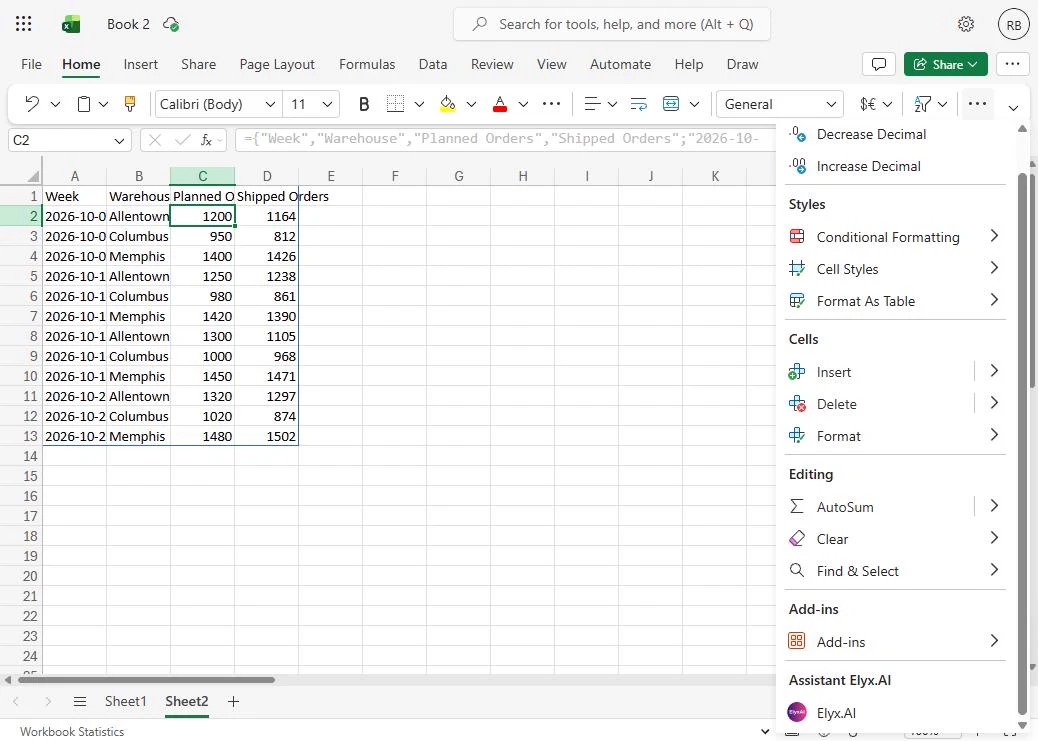
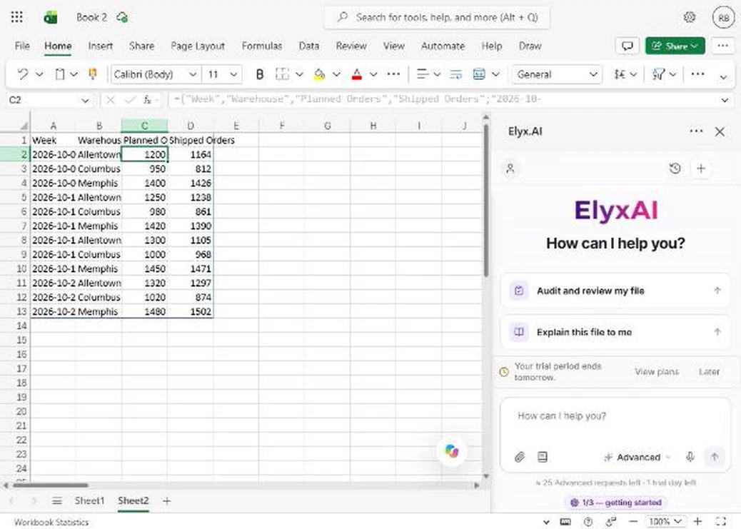
- Open the Elyx pane. You are Dana, operations manager at Northline Fulfillment, a made-up company with warehouses in Allentown, Columbus and Memphis. Every Monday you report planned vs shipped orders. Your four weeks of numbers are already on the sheet (the CSV is in the links on this lesson). On the Home tab, click ... (More options), then under Assistant Elyx.AI click Elyx.AI. On a wide screen it is a button on the Home tab.
You run operations for three warehouses, and every Monday you report planned versus shipped orders. On the Home tab, open Elyx.
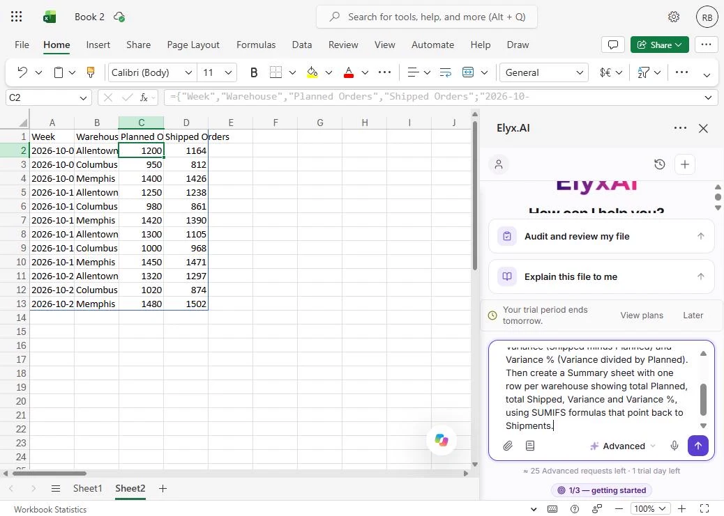
- Describe the report you want. The Elyx pane opens on the right, and shows how many requests your plan has left. Click the box and describe the whole report in one go: the two new columns, and a Summary sheet built with SUMIFS formulas. Asking for formulas, not typed-in numbers, is what makes it reusable next week.
Describe the whole report in one go. Ask for formulas, not typed-in numbers, so it works again next week.
This sheet tracks planned vs shipped orders for our three warehouses. Convert the table to plain values, rename the sheet to Shipments, and add two columns: Variance (Shipped minus Planned) and Variance % (Variance divided by Planned). Then create a Summary sheet with one row per warehouse showing total Planned, total Shipped, Variance and Variance %, using SUMIFS formulas that point back to Shipments.
- Send it. Click the purple arrow. Elyx reads the workbook, plans the changes and makes them in the open file. Ours took about a minute and a quarter.
Elyx reads the workbook, and makes the changes in the open file.
2. Build the variance report
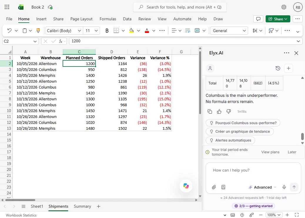
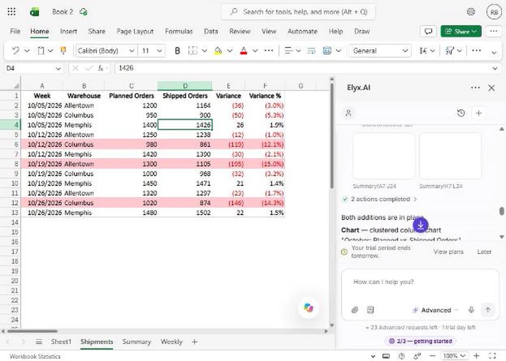
- Check the new columns. The sheet is now called Shipments, the weeks are real dates, and there are two new columns. Check one row yourself: Allentown, first week, shipped 1,164 against a plan of 1,200, so -36 and -3.0%. Negatives show in red brackets. Click the Variance columns.
Check one row yourself. Eleven sixty four shipped, against twelve hundred planned. Minus thirty six. That matches.
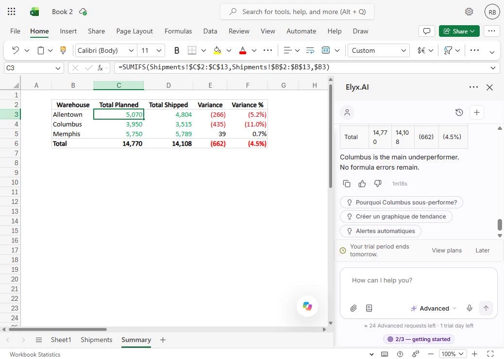
- Open the Summary sheet. Elyx also added a Summary sheet. Click its tab at the bottom.
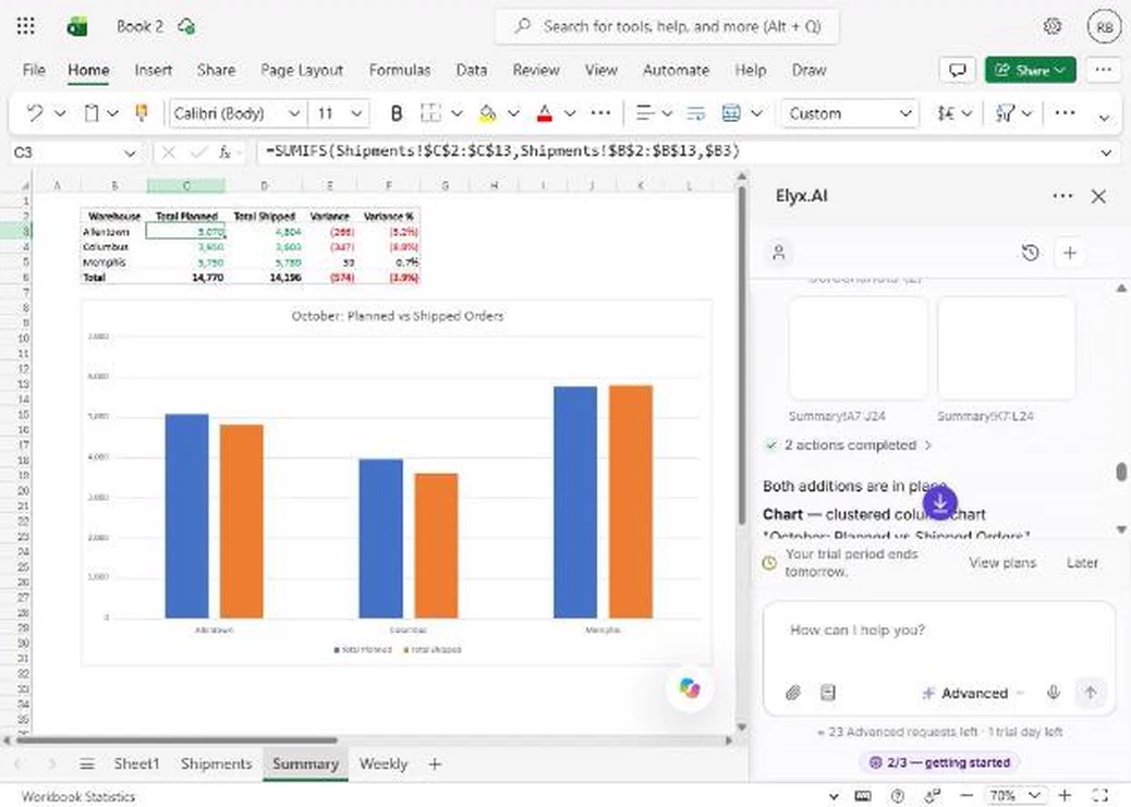
- Read the formula. One row per warehouse, with totals. Click Allentown's Total Planned and read the formula bar: =SUMIFS(Shipments!$C$2:$C$13, Shipments!$B$2:$B$13, $B3). It adds every Planned value where the warehouse matches, so the number is live. We added all three rows by hand, and they match: Allentown 5,070 vs 4,804, Columbus 3,950 vs 3,515, Memphis 5,750 vs 5,789. Click the formula bar.
Read the formula bar. It is a real SUMIFS formula, pointing back to the Shipments sheet. We added every row by hand, and they match.
3. Flag the misses
- Ask it to flag the bad weeks. Columbus is at -11% for the month. The weeks behind that are what you want to talk about on Monday. Ask for a rule, not a one-time highlight, so it keeps working when numbers change. We added Answer in English because some of Elyx's suggestions came back in French. Press Enter to send.
Ask for a rule that turns the bad weeks red. A rule keeps working when the numbers change.
On the Shipments sheet, add conditional formatting that fills the whole row light red when Variance % is worse than -10%, so the weeks where a warehouse missed plan by more than 10% stand out. Answer in English.
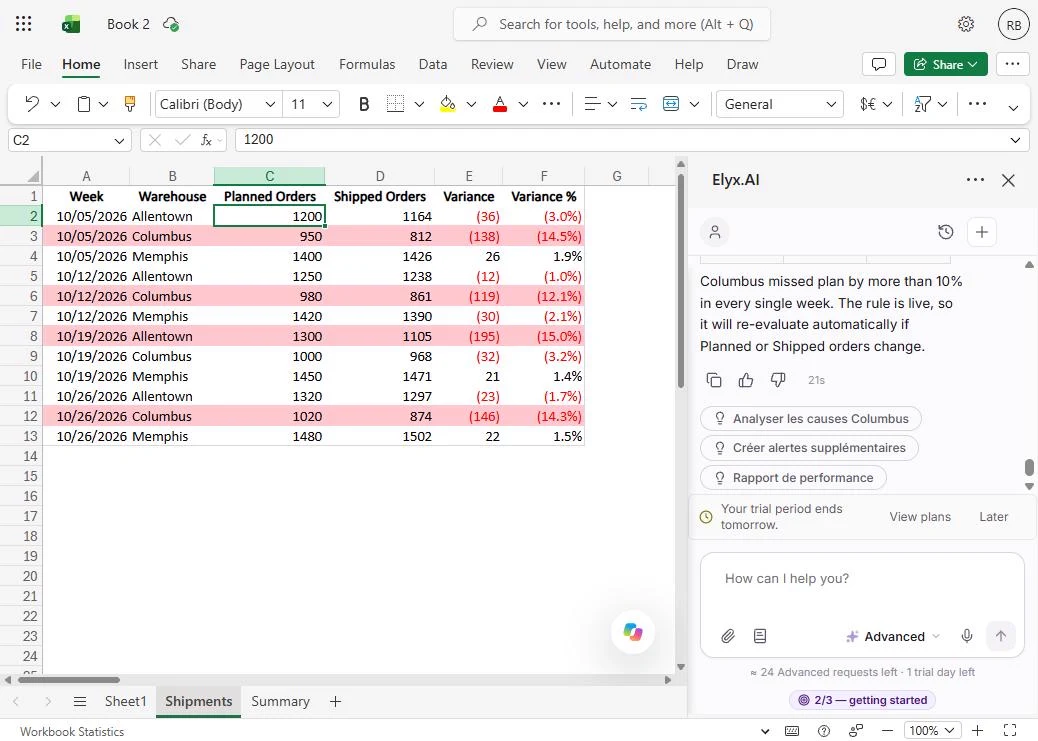
- See the flagged rows. Back on Shipments, four rows are red: Columbus in three weeks, at -14.5%, -12.1% and -14.3%, and Allentown on 19 October at -15.0%. Those are exactly the rows past -10%. Click the first red row.
Four rows turned red. Those are exactly the weeks that missed plan by more than ten percent.
- Check what Elyx says. Now read the reply. It says Columbus missed plan by more than 10% in every single week. That is not true: Columbus was -3.2% on 19 October, and that row is not red. The formatting is right and the sentence is wrong. Trust the sheet, and check any summary before you repeat it. Click the sentence.
Read the reply carefully. It says Columbus missed every week. The sheet says otherwise. The rule is right, and the sentence is wrong.
4. Make it board-ready
- Ask for a chart and a PivotTable. For the leadership call, ask for a chart of the monthly totals and a week-by-week PivotTable, in one request. Each request uses one of your plan's Advanced requests; this lesson uses three. Press Enter to send.
Ask for a chart for the leadership call, and a week by week pivot table, in one request.
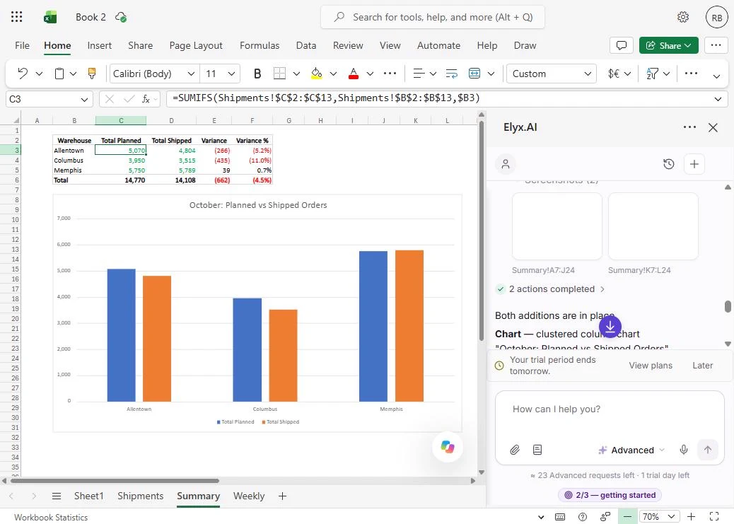
Now make it board-ready. On the Summary sheet, add a clustered column chart comparing Total Planned vs Total Shipped by warehouse, titled 'October: Planned vs Shipped Orders'. Then add a PivotTable on a new sheet called Weekly with Warehouse in rows, Week in columns and Sum of Variance as values. Answer in English.
- Look at the chart. On Summary, under the table: a clustered column chart with the title you asked for, Planned in blue and Shipped in orange. Columbus's gap is the one people will notice. Elyx also took screenshots of its own work to check it rendered. Click the chart.
Here is the chart, with the title you asked for. The Columbus gap is the one people will notice.
- Open the Weekly sheet. Click the new Weekly tab.
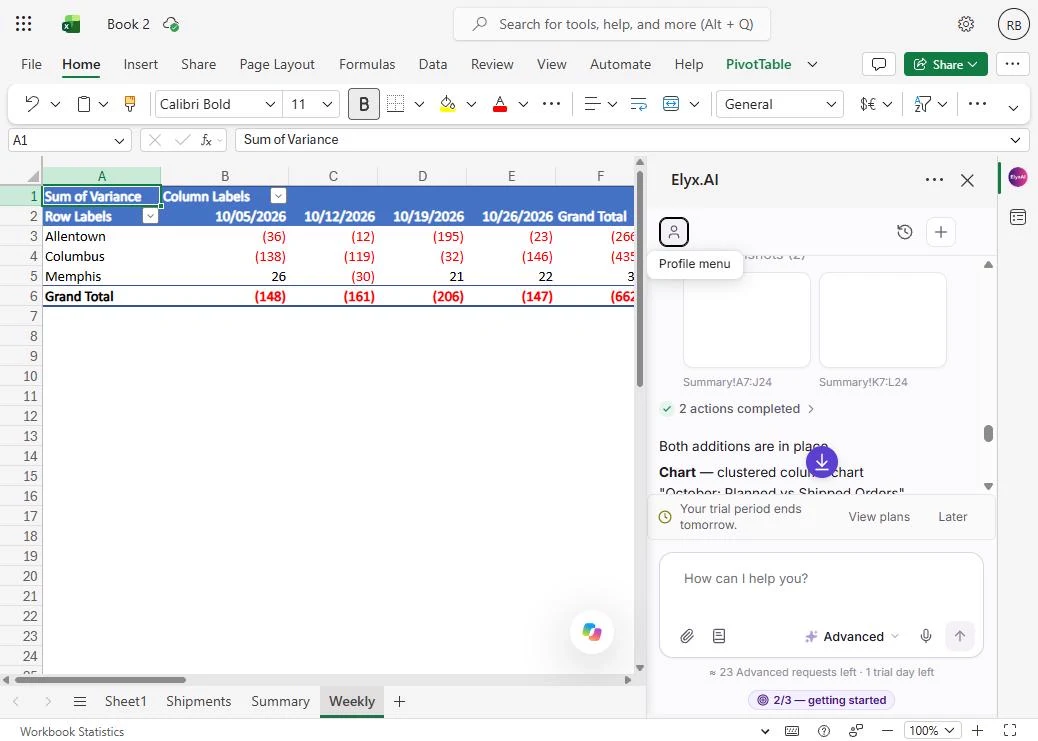
- Check the PivotTable. A real Excel PivotTable: warehouses down the side, weeks across, Sum of Variance in the cells. The grand total is (662), the same as the Summary sheet, so the two agree. 19 October was the worst week at (206). Click the Grand Total row.
A real pivot table. The grand total is minus six sixty two, the same as the summary. The two agree.
5. Rerun it next week
- Go back to Shipments. Next Monday you will paste new numbers over the old ones. Try it now with one cell. Click the Shipments tab.
Next week you will paste in new numbers. Try it with one cell.
- Change one number. Say Columbus actually shipped 900 in the first week, not 812. Click D3, type 900 and press Enter.
Say Columbus actually shipped nine hundred that week.
- Watch the row update. No new request needed. Variance is now (50), Variance % is -5.3%, and the red fill is gone, because the rule checks the value every time. Click row 3.
Variance updates, and the red fill goes away by itself. No new request needed.
- Check the Summary. Click the Summary tab.
- See the totals follow. Columbus shipped is now 3,603 and the total variance is (574): the SUMIFS formulas and the chart updated on their own. The PivotTable does not: click Data > Refresh (or right-click it and choose Refresh) after you paste new weeks. We put the number back afterwards. Click Columbus's Total Shipped.
The summary and the chart updated on their own. The pivot table needs a refresh, from the Data tab.
Screenshots
More in Business Automations
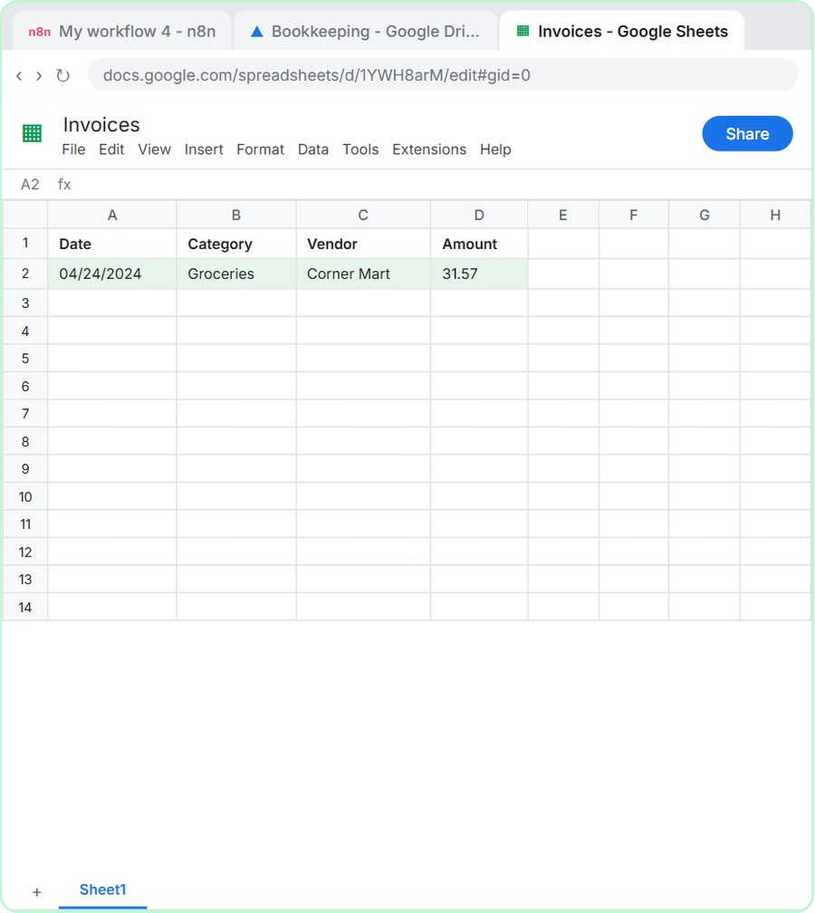 AI Receipt Extractor: Receipts to Google Sheets with n8n
Drop a photo of a receipt into an n8n chat. An AI agent reads it, pulls out the date, vendor and amount, picks a category, and adds a row to Google Sheets.
Free · Live ~12 min Intermediate
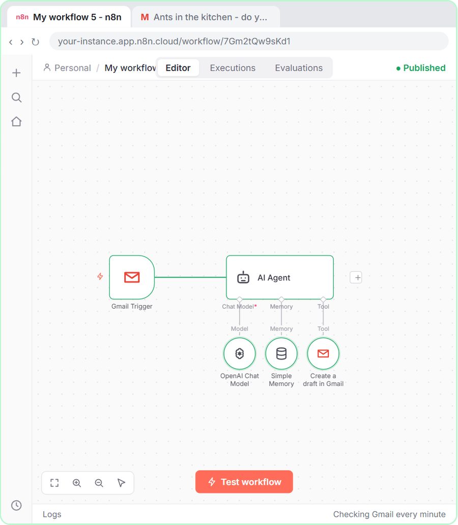 n8n AI Email Responder: Draft Gmail Replies Automatically
Build an n8n agent that watches your Gmail, reads each new customer email, and writes a reply as a draft in the same thread, ready for you to check and send.
Free · Live ~12 min Intermediate
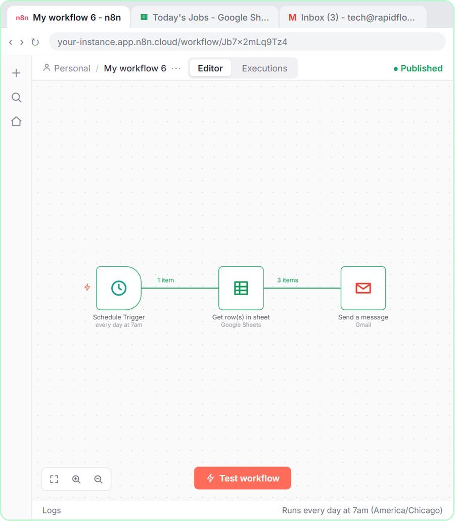 Daily Job Alerts: Email Each Tech Their Jobs from Google Sheets with n8n
Every morning at 7, n8n reads a plumbing company's jobs sheet, skips anything not assigned yet, and emails each job to the tech it's assigned to — customer, address…
Free · Live ~10 min Intermediate
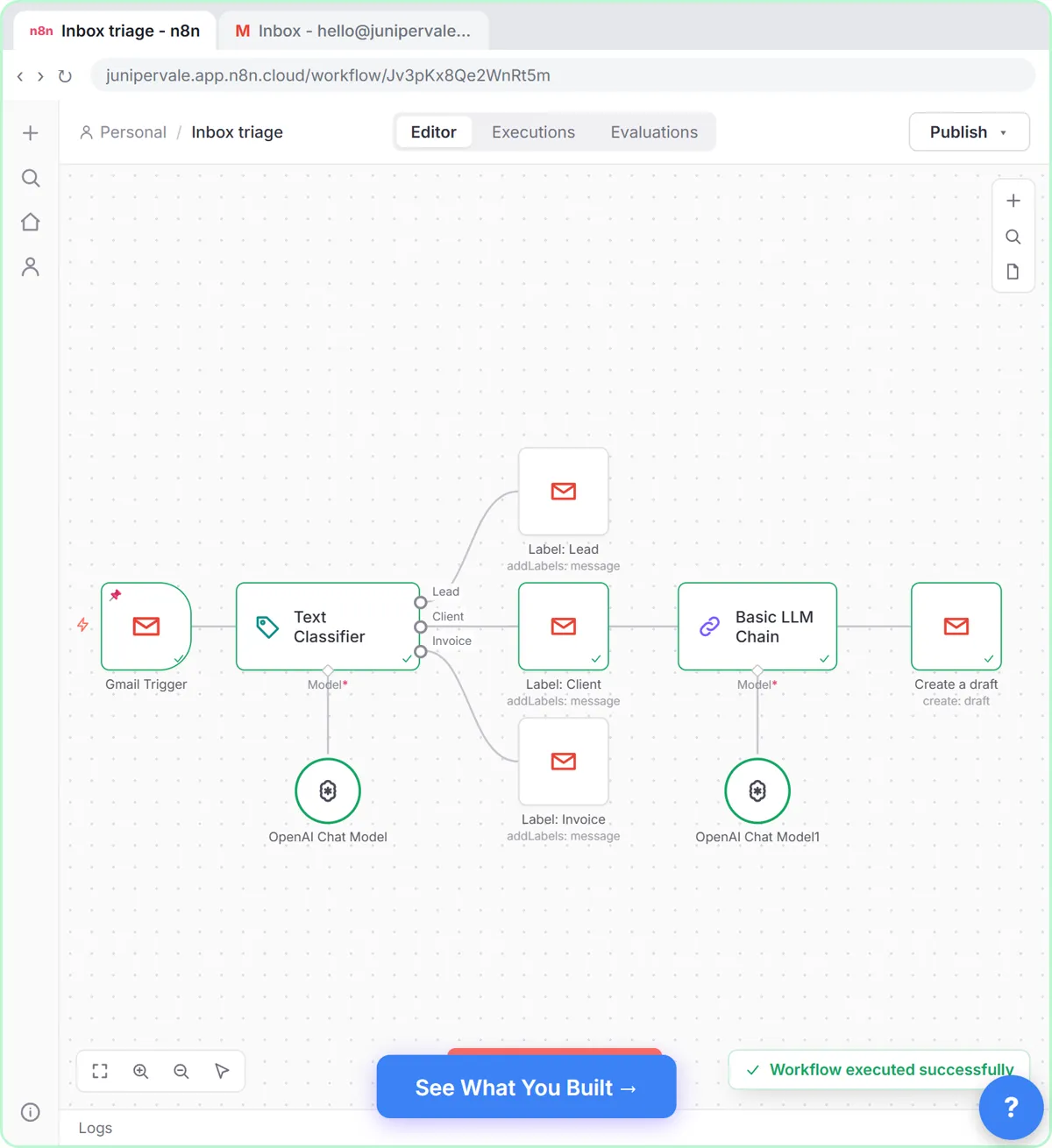 Gmail AI Triage: Auto-Label Every Email and Draft Replies
Build an n8n workflow that reads each new email, sorts it as a lead, a client or an invoice with a Text Classifier, adds the matching Gmail label, and drafts a reply to…
Free · Live ~18 min Advanced
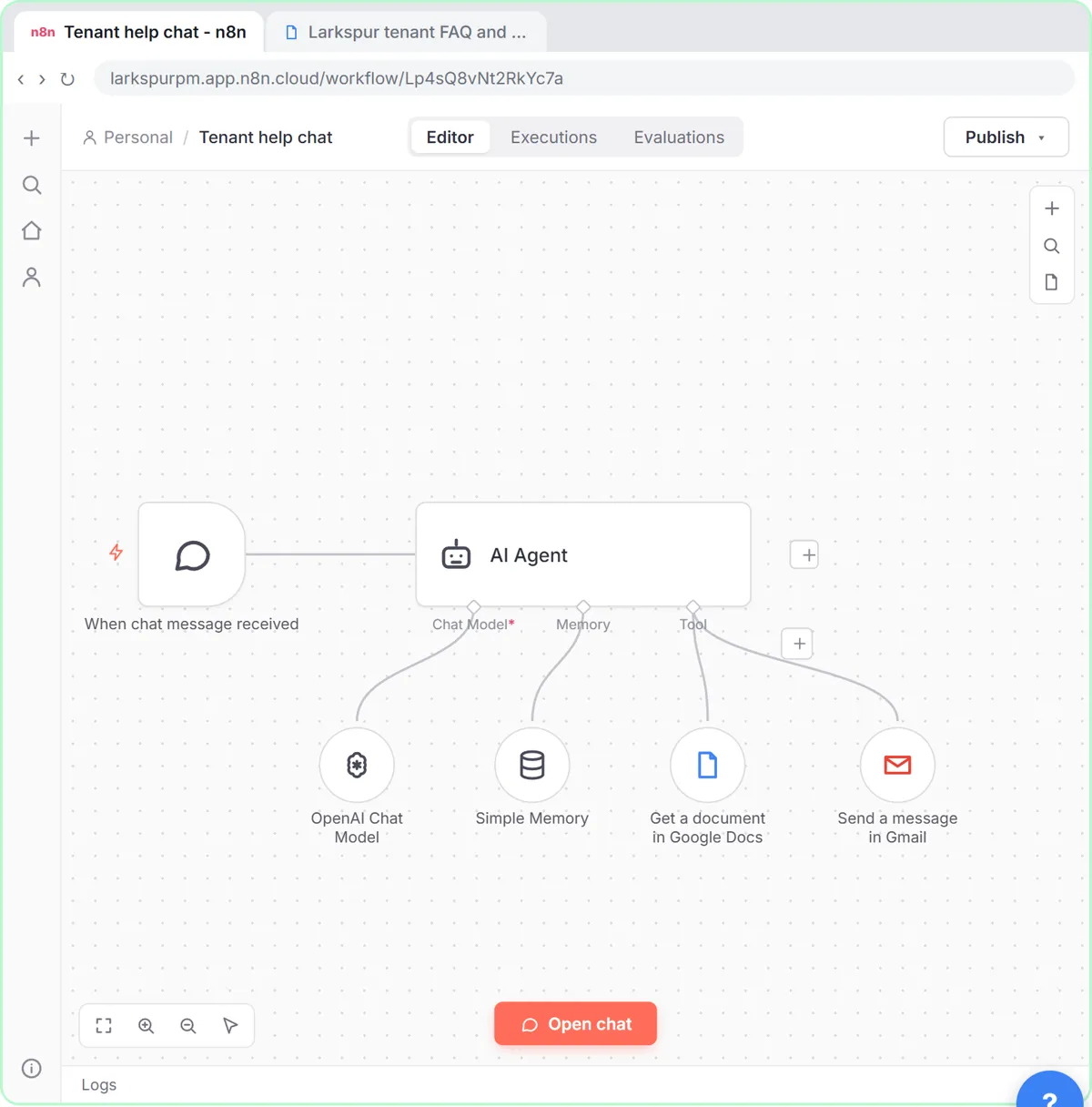 A Support Agent That Answers from Your Own Docs
Turn an n8n chat agent into a support agent that answers only from your policies in a Google Doc, refuses what it should, and hands off to a person by email.
Free · Live ~13 min Advanced
 Chatbase: Answer Customer FAQs with an AI Agent
A business case for a small firm that answers the same customer questions every week: build a Chatbase AI agent on your FAQ in the real app, make it say when it does…
Free · Live ~15 min Beginner
All 33 modules in Business Automations
Terms in this lesson
Plain-English definitions, each with an example from a free lesson.